
WRTC2014 Site Evaluation Methodology and Results
by Rich Assarabowski K1CC
This paper describes the evaluation methodology used by the WRTC2014 organizing committee to identify suitable operating sites.
The WRTC2014 Site Selection Committee made use of an analytical tool to evaluate sites as part of the search process to find 65 suitable sites. The need for such a tool became very obvious after a few early attempts at deciding whether a site would be acceptable or not. First of all, there is no ideal level ground in New England (except over water!). Second, every location will have varying terrain in different directions. It quickly became apparent that intuition does not work in comparing sites to each other.
A valuable tool for such an analysis is to use N6BV’s High Frequency Terrain Assessment (HFTA) model (Ref. 1). This ray-tracing program uses the terrain profile in a given direction to generate an antenna pattern over the actual topography and then compares it against a statistical distribution of arrival angles for a given target area (e.g. Europe, US, etc.) and calculates a figure of merit (FOM) in dBi. This figure of merit is a weighted average of antenna gain over the range of expected arrival angles for that particular target area. Typical use of HFTA is to optimize antenna heights at a particular location. In our situation, the antennas were fixed and we used the model to evaluate station locations.
The essence of the WRTC2014 terrain analysis methodology is to perform the following for each site:
- Calculate the FOM for a given direction and band over the actual terrain profile.
- Calculate the FOM for the same direction and band over flat ground.
- The difference between (1) and (2) yields the FOM for that direction and band.
An ideal WRTC site would have an FOM of 0.0 in each direction for each band. Since this is highly unlikely except on water, we defined two critical directions for WRTC; Europe (45°) and the US. Because the US covers a wide azimuthal range, we calculated the US FOM as the average of the FOMs at 210° (US Southeast) and 270° (US West Coast).
Our sites often showed significant variation in FOM between bands and directions. Some bands and directions are clearly more important than others. The solution was to weigh the contribution of each band/direction to the final score.
What about other directions? During our site search, we checked to make sure there were no significant hills or slopes in other directions but did not model them. It would simply have taken too much time and would require additional assumptions regarding the contribution of these other directions to the final score which essentially yield only multipliers.
In 2012, in order to estimate a detailed breakdown of a winning WRTC2014 score, we surveyed Committee members and came up with a set of band-weighting factors. A comparison of the predicted winning score from 2012 and the actual winning score of N6MJ and KL9A shows good correlation (see http://konecc.wix.com/HFTA). The bottom line is that we predicted that approximately 80 percent of the score (not number of QSOs) would derive from the European direction and approximately 20 percent from the US direction.
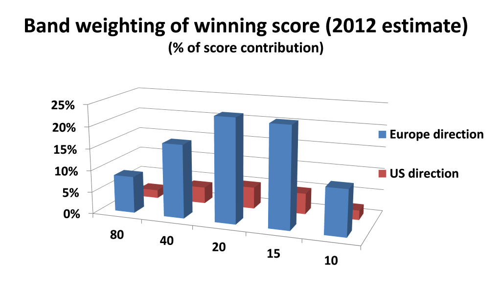
Figure 1. Estimated score contribution of each band and direction
The composite (or overall) figure of merit (FOM) is then calculated as a weighted average of the FOM toward Europe and the United States for each band. These calculations were done for each candidate site and for various antenna locations as they evolved. The various shades on the table made it easy to spot outliers. A perfect site would be close to 0.0 (white), with darker shading corresponding to a higher FOM.
Figure 2 offers an example of FOM results for 15U (Myles Standish) where the K1A team operated in 2014. Note in this example that even though the US FOM is 0.9, it only added 0.1 to the overall FOM. The US direction is just not that important in the IARU contest from New England. Our objective in the analysis, therefore, was to find sites that would be as close to flat as possible using this overall FOM as a figure-of-merit.
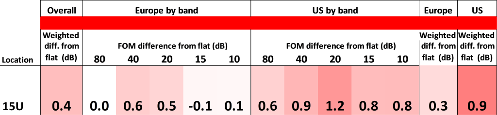
Figure 2. FOM table for site 15U (Myles Standish)
We performed a sensitivity analysis to see how the FOM would change if the WRTC stations worked a lot more US stations. The change in FOM was only a few tenths of a decibel for most sites and would have not affected our site selection.
The remaining issue was where to draw the line for rejecting locations as being too good or too poor. In 2012 I made a presentation at the New England Division Convention at Boxboro, Massachusetts, laying out the guidelines we wanted to follow:
- The FOM difference from flat terrain shall not exceed 3 dB on any one band to either the US or Europe.
- The maximum weighted FOM difference from flat terrain for either the US, Europe or both should not exceed 1.8 dB.
- Gain for a range of 4-5 elevation angles should not differ by ~8–10 dB from flat terrain on any band to either the US or Europe (ie, no big peaks or valleys in the antenna pattern).
- The overall FOM weighted difference from flat terrain shall not exceed 1.5 dB.
An easy way to translate these guidelines into more intuitive parameters is to convert them to power levels. For example, a 1.5 dB difference from flat terrain would be equivalent to a station running 140 W instead of the 100 W limit.
There were many sites along the way that exceeded these limits and were rejected. Most of our final sites, but not all, were within these self-imposed limts that we defined as objectives back in 2012. It was either that or simply not have 65 sites for the contest.
Topographic Database Considerations
A step-by-step procedure and templates for the WRTC terrain analysis is available on http://konecc.wix.com/HFTA . A very nice tool for quickly visualizing terrain is at http://www.geocontext.org/publ/2010/04/profiler/en/ which uses the NED topographic database. The software can generate CSV files which can be converted for use with HFTA.
The first step in any terrain analysis is to have a good map of the area. We used http://mapper.acme.com/ for all of our site layouts. It is based on Google Maps, but offers a unique instant overlay of a US Geological Survey (USGS) topographic map (for the US only) at a mouse click. This makes it very easy to quickly “eyeball” locations without running a detailed terrain model.
Next, we needed to establish a credible topographic database for New England. N6BV suggested the digital elevation model (DEM) database is usually the most accurate within the US. The Reagan-era motto “trust but verify” led me to pick several test sites to give me confidence in the model. One of the Wrentham sites (10A) was a good one. The terrain has a very slight downslope toward Europe, is relatively flat to the southwest and flat to the west, but then dropping rapidly toward a lake. With Dean’s help, we generated National Elevation Dataset (NED), DEM, and shuttle radar topography mission (SRTM) databases. I painstakingly compared the profiles in various directions using USGS maps as a benchmark. The lake to the west of 10A was a good reference point. The terrain profiles did not always accurately define the edge of the lake, and in some of the terrain databases, the terrain over the lake was not flat(!). After due consideration, I selected the NED for our WRTC analysis.
Assumptions and Limitations
Our methodology incorporated multiple assumptions. One of the biggest unknowns is the arrival angle distribution used in the model. We used N6BV’s published arrival angle distributions for each target area (Europe and the US) which are based on VOACAP predictions. The supporting data for these elevation angle statistics is acknowledged to be weak but it’s the best we have (Ref. 2). In addition, arrival angles can be very different depending on the Solar Spot Number (SSN), geomagnetic disturbances, season, and time of day. The VOACAP does not calculate arrival angles for Es and double-hop Es propagation which frequently occurs in summertime propagation. Given the absence of any better data, this is what we used and it was a reasonable choice in predicting propagation two years prior to the event.
Here is a list of other considerations and observations made as a result of running HFTA hundreds of times over the course of 2½ years:
- When examining HFTA plots, it is very important to realize that there are artifacts in the calculations. One must not try to interpret small peaks and valleys in the antenna response curve as necessarily being significant. A good example of that is the Mansfield airport location (12A), where small dips in the antenna response happen to coincide with peaks in the arrival angles, leading to an overall FOM of -0.3, making the site model appear worse than it actually is. Real-world peaks and valleys in antenna response are much “smoother” than the model shows. Any micro-analysis of these small perturbations is beyond the resolution of this model and the underlying terrain database.
- The HFTA results can be very sensitive to terrain data across different databases (NED, DEM, etc). Running sensitivity tests with small perturbations in antenna location, terrain files and azimuth for some of the sites occasionally showed a significant variability in results, especially on hilly and bumpy terrain.
- Intuition regarding the effects of terrain on antenna pattern is not very reliable. The effect of terrain on a 40 foot high antenna is much different than it is on a 100 foot antenna. Local terrain features (saddlebacks, humpbacks) within the ground reflection zone can sometimes result in very large gain differences over a narrow range of radiation angles. HFTA has been used very successfully by station designers, but it is not a rigorously validated model.
- We used the default distance for terrain profiles (4400m) as recommended by N6BV for general use. However, my own empirical observation after making hundreds of runs, the ground reflection zone for a small 40 ft high antenna is no more than 1000m for all practical purposes. There may be secondary reflections occurring due to diffraction over the bumpy terrain at distances >1000m. Terrain beyond 1000m is of not much consequence at these low antenna heights (Ref. 3). Careful study of the terrain profiles and HFTA plots will bear this out.
- There can be significant diffraction effects over bumpy terrain we encountered in many of our sites. Turning diffraction on and off in HFTA illustrates this vividly. This further complicates any intuitive predictions of how well a site will perform.
- HFTA does not work with vertical polarization. The inverted-V’s on 80 and 40 have a vertical polarization component which is not accounted for in the model.
- Man-made features such as fill for roads can distort the results somewhat. This was the case, for example, at Hollis (1A) where the actual antenna location on a recently constructed sports field is not reflected accurately in the terrain database.
Terrain Data and HFTA Plots
All terrain profiles and antenna patterns for each of the 59 teams are available at WRTC2014 terrain and HFTA data 13_Aug_2014 (Ref 4). For each site, the terrain profile is shown followed by HFTA plots, for both Europe and for the two US directions. For the US, the blue curves are for 270 deg and the red for 210 deg. Note that the Rice sites (11B, 11C and 11E) are labeled as “Wrentham”, which was our internal designation for this property, so this is not an error. All terrain plots have been adjusted to the same scale so they can be easily compared.
Comparison of Model to Final Results
A comparison of final scores with the overall FOM for each of the sites is shown in Figure 3.
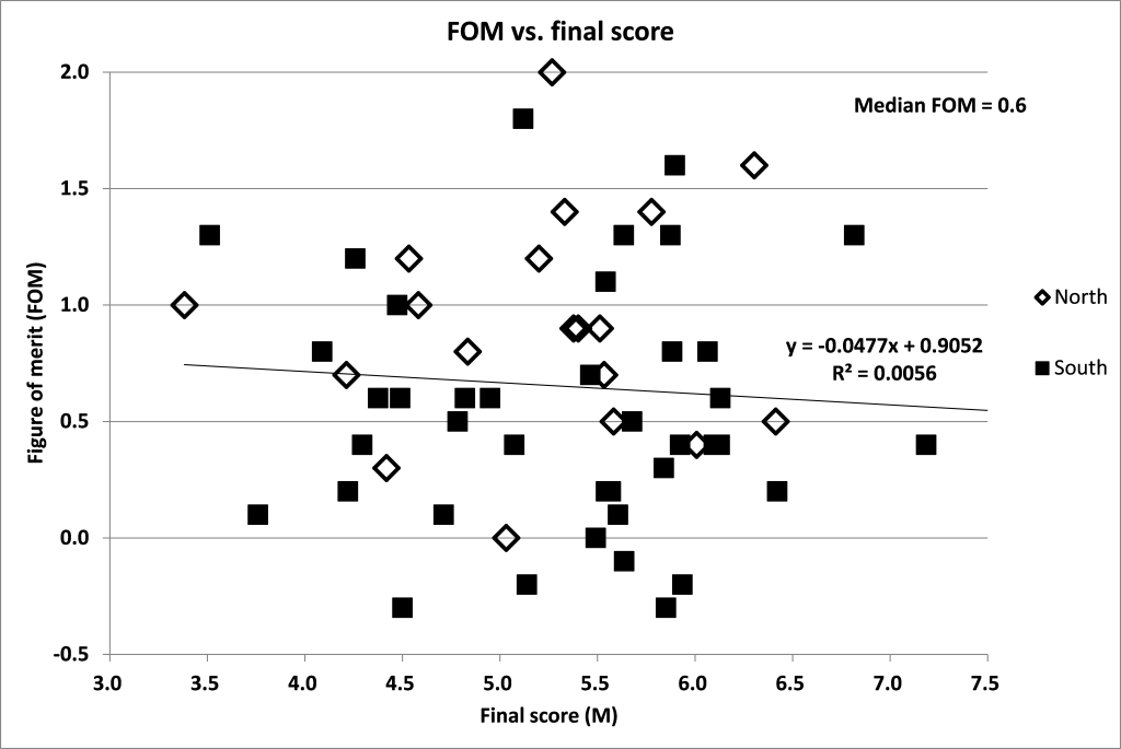
Figure 3. FOM vs Final Score
There is no correlation to the final score as seen by the linear regression analysis (R2 = 0.0056). A perfect correlation would give an R2 of 1.0. The range of FOM was from -0.3 to 2.0. The highest FOM site was Twin Valley (FOM was 2.0) which was a spare site pressed into service at the last minute. The median FOM of all the sites was 0.6. The plot of just the top 20 scores and their station calls signs also shows no obvious terrain advantages.
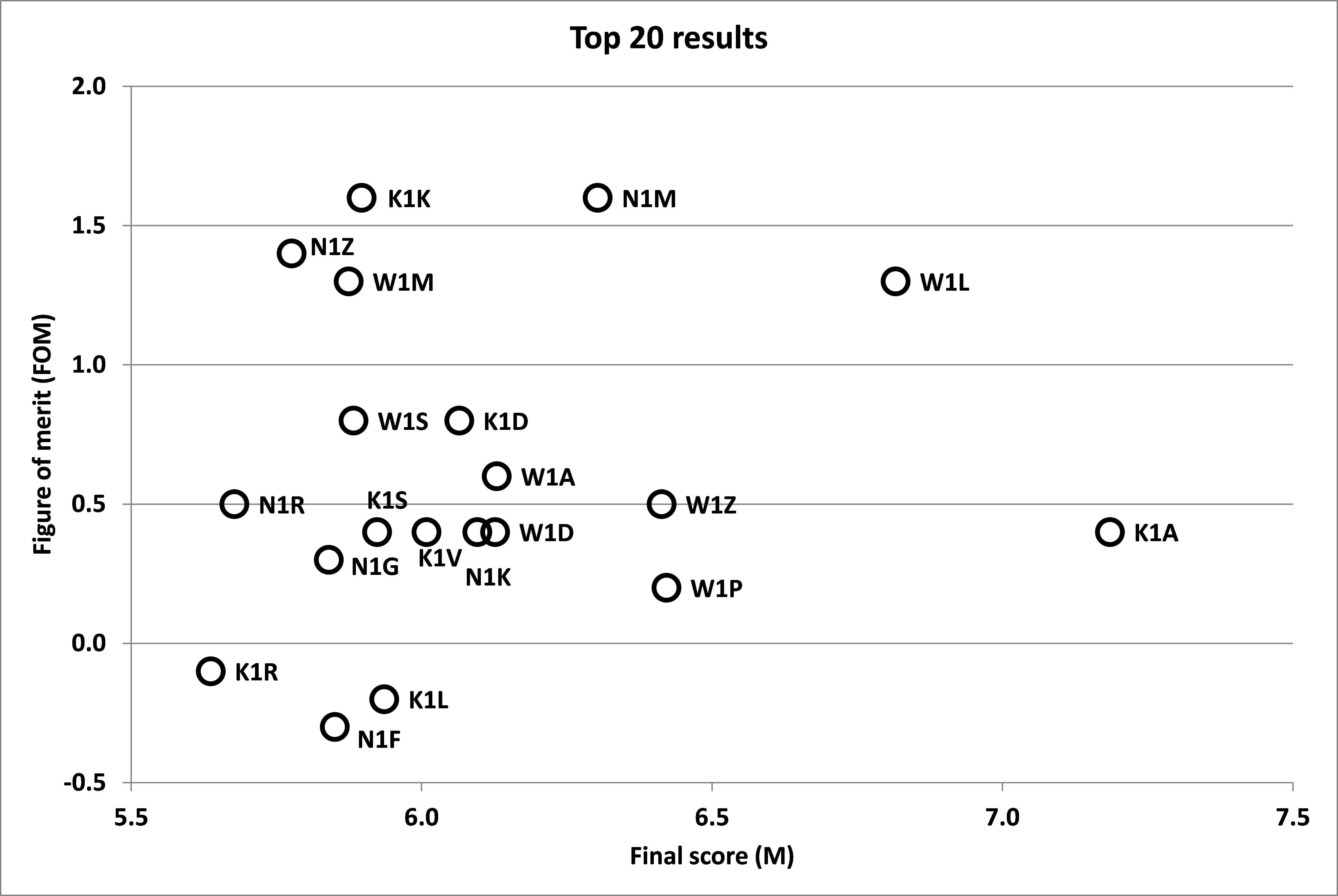
Figure 4. FOM vs Score for top 20
See the map at http://www.wrtc2014.org/map-of-operating-sites/ for the location of all operating sites.
Site Comparisons
The tables below show each of the 59 sites and their calculated FOMs.
North Sites
| Site | Call | Operators | Coordinates | Overall Weighted diff. from flat (dB) |
Europe Weighted diff. from flat (dB) |
US Weighted diff. from flat (dB) |
| 01A | W1T | AD4Z W4UH | N 42.73222 W 71.59279 | 1.2 | 1.5 | -0.4 |
| 02A | W1Z | N5DX N2IC | N 42.70303 W 71.58863 | 0.5 | 0.6 | 0.5 |
| 02B | W1U | LZ4AX LZ3FN | N 42.70127 W 71.57982 | 0.9 | 1.1 | -0.2 |
| 03A | K1U | KF5EYY YT1AD | N 42.68956 W 71.59410 | 1.0 | 1.2 | 0.1 |
| 04A | N1M | K9VV VE3EJ | N 42.66727 W 71.62870 | 1.6 | 1.8 | 0.2 |
| 04B | K1Z | VE7CC VE7SV | N 42.67007 W 71.62269 | 1.4 | 1.6 | 0.3 |
| 05A | K1W | K6AM N6AN | N 42.68618 W 71.59022 | 2.0 | 2.3 | 0.2 |
| 05B | N1T | ES5TV ES2RR | N 42.68117 W 71.58812 | 0.9 | 1.2 | -0.8 |
| 06B | K1C | KE3X K0DQ | N 42.52024 W 71.60899 | 0.9 | 0.9 | 0.9 |
| 06C | W1F | CT1ILT CT1BOH | N 42.54489 W 71.62133 | 0.0 | 0.0 | 0.0 |
| 06D | N1V | K7RL KL2A | N 42.54663 W 71.63347 | 1.2 | 1.4 | 0.3 |
| 06E | K1V | G0CKV M0DXR | N 42.53472 W 71.63042 | 0.4 | 0.3 | 0.9 |
| 06G | N1D | NR5M W2GD | N 42.53492 W 71.60117 | 1.0 | 1.1 | 0.3 |
| 06H | K1F | VY2ZM KK6ZM | N 42.54787 W 71.61504 | 0.7 | 0.7 | 0.5 |
| 06J | N1Z | PY1NX LZ3YY | N 42.52311 W 71.60373 | 1.4 | 1.5 | 0.9 |
| 06K | K1I | UU4JMG UU0JM | N 42.54299 W 71.63744 | 0.5 | 0.2 | 2.0 |
| 06Q | W1N | 5B4WN 5B4AFM | N 42.54138 W 71.60629 | 0.8 | 0.8 | 0.5 |
| 07B | K1P | M0CFW GI0RTN | N 42.48372 W 71.77833 | 0.7 | 0.5 | 1.6 |
| 07C | N1P | CX6VM LU1FAM | N 42.48904 W 71.77934 | 0.3 | -0.3 | 2.3 |
South Sites
| Site | Call | Operators | Coordinates | Overall Weighted diff. from flat (dB) |
Europe Weighted diff. from flat (dB) |
US Weighted diff. from flat (dB) |
| 08A | K1M | IK1HJS I4UFH | N 42.21484 W 71.33339 | 1.3 | 1.5 | -0.1 |
| 08B | N1A | DL1QQ DL8DYL | N 42.20961 W 71.33097 | 1.3 | 1.6 | -0.4 |
| 08C | W1R | OH2BH OH2MM | N 42.21174 W 71.33778 | -0.3 | -0.7 | 1.3 |
| 08D | W1M | 4O3A HA1AG | N 42.20899 W 71.34627 | 1.3 | 1.6 | -0.2 |
| 09A | N1O | RC9O UA9PM | N 42.21764 W 70.83317 | 0.7 | 0.9 | -0.3 |
| 09B | W1W | OH2UA OH6KZP | N 42.21911 W 70.84024 | 0.2 | 0.2 | 0.3 |
| 09D | K1G | 9A6XX 9A1UN | N 42.22343 W 70.84605 | 1.1 | 1.3 | 0.1 |
| 09F | K1O | JH5GHM JA1OJE | N 42.21499 W 70.85559 | 0.1 | 0.1 | 0.1 |
| 09G | N1L | KU1CW EA5GTQ | N 42.21324 W 70.84757 | 1.8 | 2.2 | -0.5 |
| 09H | N1R | UA3DPX UA4FER | N 42.18258 W 70.84749 | 0.5 | 0.6 | 0.1 |
| 10A | W1B | OE2VEL OE5OHO | N 42.08580 W 71.32105 | 0.6 | 0.7 | 0.4 |
| 10F | W1D | K1LZ YT6W | N 42.08238 W 71.32759 | 0.4 | 0.4 | 0.5 |
| 10G | K1K | RL3FT RA3CO | N 42.09002 W 71.31741 | 1.6 | 1.8 | 0.3 |
| 11B | N1G | RX3APM RV1AW | N 42.07739 W 71.32641 | 0.3 | 0.1 | 1.0 |
| 11C | K1D | UR0MC VE3DZ | N 42.07470 W 71.32142 | 0.8 | 0.8 | 0.9 |
| 11E | W1S | F8DBF F1AKK | N 42.07891 W 71.31810 | 0.8 | 1.0 | 0.0 |
| 12A | N1F | RW1A RA1A | N 41.99903 W 71.19228 | -0.3 | -0.3 | 0.2 |
| 12D | K1N | OE3DIA E77DX | N 41.99997 W 71.20113 | 0.1 | 0.0 | 0.2 |
| 13A | K1R | N4YDU N3KS | N 41.88059 W 70.99020 | -0.1 | -0.5 | 1.3 |
| 13B | W1G | F4DXW F8CMF | N 41.87113 W 70.98153 | 0.5 | 0.5 | 0.5 |
| 14A | W1L | OM3BH OM3GI | N 41.78610 W 71.05130 | 1.3 | 1.6 | 0.0 |
| 14C | N1K | DK6XZ DK9IP | N 41.81255 W 71.10927 | 0.4 | 0.5 | 0.1 |
| 14D | W1A | LY9A LY4L | N 41.83188 W 71.11659 | 0.6 | 0.7 | 0.2 |
| 15A | W1C | 9A5K 9A1TT | N 41.83721 W 70.65687 | 0.2 | 0.2 | 0.5 |
| 15B | W1O | OM2VL OM3RM | N 41.83365 W 70.65223 | 0.6 | 0.7 | 0.0 |
| 15C | W1K | BA5CW BA7IO | N 41.83503 W 70.64477 | 0.8 | 0.9 | 0.4 |
| 15D | W1I | W2RE WW2DX | N 41.83039 W 70.64612 | 0.4 | 0.4 | 0.4 |
| 15E | K1S | W2SC N2NL | N 41.83243 W 70.65804 | 0.4 | 0.4 | 0.3 |
| 15F | K1L | S50A S57AW | N 41.84834 W 70.69252 | -0.2 | -0.4 | 0.4 |
| 15G | K1T | IZ1LBG WQ2N | N 41.81350 W 70.67121 | 0.0 | 0.0 | 0.1 |
| 15H | N1N | KH6ND KH6SH | N 41.84928 W 70.68134 | 1.2 | 1.4 | 0.3 |
| 15I | N1U | K8MR K9NW | N 41.84859 W 70.67522 | -0.2 | -0.1 | -0.4 |
| 15J | N1B | YL1ZF YL2GQT | N 41.81724 W 70.67938 | 0.6 | 0.7 | 0.2 |
| 15M | N1W | PY2YU PY2NDX | N 41.86035 W 70.66443 | 0.4 | 0.3 | 0.6 |
| 15N | K1B | W9RE N5OT | N 41.85969 W 70.67053 | 0.2 | 0.0 | 1.0 |
| 15O | W1V | R9DX UA9CDV | N 41.85283 W 70.67272 | 0.6 | 0.5 | 0.9 |
| 15P | N1S | LX2A YO3JR | N 41.85925 W 70.68597 | 0.1 | 0.1 | 0.0 |
| 15R | N1C | IK2NCJ IK2QEI | N 41.85886 W 70.67814 | 1.0 | 1.1 | 0.6 |
| 15U | K1A | N6MJ KL9A | N 41.82532 W 70.64618 | 0.4 | 0.3 | 0.9 |
| 15W | W1P | DJ5MW DL1IAO | N 41.82787 W 70.65786 | 0.2 | 0.1 | 0.4 |
REFERENCES
- The software comes on a CD with purchase of the ARRL Antenna Book
- See http://www.voacap.com/angle.html for an excellent discussion of arrival angles in VOACAP
- See http://www.vk3um.com/Ground%20Gain_DUBUS%203-2011_ON4KHG.pdf for more detail on basic ground reflection theory
- Terrain profiles and antenna elevation angle patterns for each of the 59 competition sites are available at WRTC2014 terrain and HFTA data 13_Aug_2014 Note: This pdf file is easier to view in Adobe Acrobat reader than in your browser. Right click on the link and select Save As… to copy to your computer. Then double click on the file to view.